
The book
Chapter 2: Field Mechanics of the Supertoroid
The geometry of the two circulations, the safety factor, and J. B. Taylor’s model of relaxation toward unclenched flow.
2.1 The Topology of Recurrence: Why a Sphere Cannot Breathe
If Nāgārjuna and Bateson have cleared away our habit of dividing the world into rival substances, we are left with a practical architectural question: What is the actual shape of an undivided, self-sustaining process?
For over two thousand years, from Parmenides and Plato down to early twentieth-century atomic models, the Western imagination was hypnotized by the sphere (). The sphere was revered as the emblem of perfection because every point on its surface sits at an equal radius from a static, unmoving center. Yet the sphere suffers from a fatal dynamic defect. By the Hairy Ball Theorem of algebraic topology (proven by Brouwer in 1912), you cannot comb a continuous, non-vanishing tangent vector field flat across the surface of a sphere without creating at least one singular point—a cowlick or stagnant pole where the flow stops dead or tears loose from the surface. A sphere is a monument to static containment; it is a terrible vessel for continuous, unhurried circulation.
The moment a physical system commits itself to continuous, self-renewing flow—whether it is a smoke ring rising in still air, a magnetic confinement vessel in a fusion laboratory, a Bénard convection cell, or the speculative cosmological ovoid proposed last year by Itzhak Bentov in Stalking the Wild Pendulum—nature abandons the sphere and adopts the torus ().
Why does a circulating process demand a torus? Because a torus is the simplest closed, orientable manifold in three-dimensional space upon which a continuous vector field can flow forever without ever encountering a dead-end pole or an arbitrary wall. It possesses Euler characteristic zero (). It takes what appears to be an "inside" (the central vertical throat) and turns it seamlessly into an "outside" (the overarching return mantle) solely through the continuity of movement.
Before we allow this geometry to serve as a contemplative mirror for a human life, we must honor the discipline of the physicist and state the mathematics of the nested torus—and its magnetohydrodynamic field equations—with absolute precision. A metaphor that blurs its own mathematical foundations cannot carry the weight of a life. Let us establish the geometry first, distinguish the exact physical assumptions required to put a field in motion upon it, and only then examine how a life of work and presence maps onto its coordinates.
2.2 Differential Geometry of the Nested Manifold (The Supertoroid)
In the popular parlance of our coastal seminars, one often hears talk of "a torus within a torus." Yet that phrase is mathematically ambiguous unless we specify which of at least four distinct geometric structures we mean:
1. Concentric Nested Toroidal Surfaces: A continuous family of non-intersecting toroidal shells sharing a common major axis and major radius , parameterized by a varying minor radius .
2. Linked Vortex Rings: Two or more discrete toroidal tubes looped through one another like links in a chain, each circling the other’s core.
3. A Toroidal Helix (Coil on a Core): A secondary smaller tube wound helically around the surface of a primary toroidal ring.
4. Deformed Cross-Sectional Tori: Surfaces whose cross-sections depart from a true circle through higher-order shape exponents.
Throughout this treatise, when we use the term supertoroid, we define it specifically as the union of a family of concentric nested toroidal flux surfaces (Type 1) coupled dynamically to internal poloidal and secondary recirculating sub-loops (Types 2 and 3) via field superinsertion.
Let us construct the primary nested manifold in three-dimensional Euclidean space with Cartesian coordinates . Let be a fixed constant representing the major radius—the distance from the origin at the center of the central opening out to the circular spine (the magnetic axis) of the tube. Let be the minor radius, measuring the radial distance outward from that circular spine toward the skin of the tube, subject to the strict geometric bound so that the inner throat remains open.
A standard ring torus of fixed minor radius is parameterized by two independent angular coordinates, and :
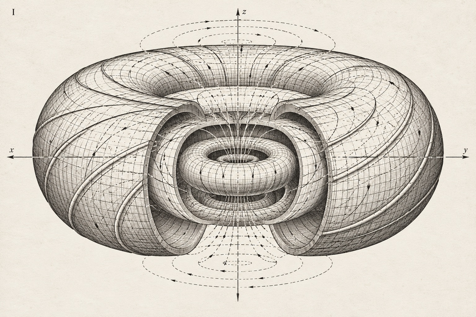
Let us examine the physical meaning of the three coordinates :
The Toroidal Angle (): This angle runs horizontally all the way around the central vertical -axis. It governs the grand revolution of the ring as a whole.
The Poloidal Angle (): This angle runs around the small circular cross-section of the tube itself, passing through the inner throat (at , where the distance from the -axis is minimal, ), arching over the top crown (), sweeping down the outer equator (, where distance from the -axis is maximal, ), and curving underneath () to re-enter the throat.
The Radial Foliation Parameter (): When we hold fixed at some value , the mapping sweeps out a single two-dimensional toroidal surface of topology . When we allow to vary continuously across the open interval (where is the outer containment boundary of the vessel), the mapping generates an infinite family of concentric, nested toroidal surfaces filling the solid torus. In this idealized geometric family, distinct surfaces and never intersect one another ().
To perform vector calculus on this nested manifold, we compute the covariant tangent basis vectors by taking the partial derivatives of the position vector with respect to each coordinate:
Taking the dot products , we observe immediately that the off-diagonal terms vanish (). Thus forms an orthogonal curvilinear coordinate system with the Riemannian metric tensor:
From the square roots of the diagonal metric components, we obtain the scale factors (Lamé coefficients) , , and , along with the differential volume element:
Normalizing the tangent vectors by their scale factors yields the local orthonormal basis triad at every point inside the supertoroid:
Notice a vital geometric feature encoded in the scale factor . On the outer equator of the torus (), the path length around the major axis is long (), and the Gaussian curvature of the surface is positive, like an apple skin. On the inner throat facing the central hole (), the path length is compressed (), and the Gaussian curvature is negative, like a mountain pass or saddle:
Every particle or field line executing a poloidal turn () must alternately expand across the outer world of positive curvature and compress through the high-density, saddle-curved throat near the central axis.
2.3 Adding a Field: Flux Surfaces, Helical Winding, and the Safety Factor $q$
Up to this point, we have written pure geometry. A surface equation supplies shape, but shape alone does not move a speck of dust or sustain a single thought. To turn geometry into physics, we must supply a vector field (giving direction and magnitude at every point), evolution equations, boundary conditions, material properties, and energetic forcing.
In 1970, when the Swedish physicist Hannes Alfvén accepted the Nobel Prize in Physics for his foundational work in magnetohydrodynamics (MHD), he reminded the scientific community in his lecture ("Plasma Physics, Space Research and the Origin of the Solar System") that magnetized plasmas—conducting fluids threaded by magnetic fields—behave in ways that flatly contradict the intuition of empty-space mechanics. When an ionized gas or conducting fluid moves through a magnetic field, the field lines are not passive imaginary chalk marks; they carry tension like stretched elastic bands and exert lateral pressure against neighboring lines.
Suppose we fill our solid torus with a magnetized plasma and establish a family of nested magnetic flux surfaces. We label each nested surface by a smooth scalar flux function (where, in the simplest axisymmetric circular case, depends only on the minor radius ). The gradient vector points strictly normal (perpendicular) to each nested surface, along .
For the magnetic field to remain confined upon these nested surfaces without leaking across them toward the outer wall, the radial component must vanish everywhere. Mathematically, this is stated by the fundamental tangency condition:
When holds throughout the volume, every magnetic field line lies wholly upon a single nested surface . Using our local orthonormal basis , any magnetic field satisfying this condition decomposes purely into two tangent components:
where is the poloidal magnetic field (generated primarily by electric currents flowing toroidally around the main ring) and is the toroidal magnetic field (generated primarily by external or poloidal currents wrapping around the tube).
Now ask: Why do we need both and ? Why not simply run a pure toroidal field in a simple circle around the main ring?
Every plasma physicist learns the answer in his first week at the tokamak or pinch bench: a pure toroidal field cannot maintain equilibrium! Because the toroidal field lines curve around the -axis with radius , the magnetic field is stronger near the inner throat () and weaker at the outer equator. This radial field gradient () combined with line curvature causes positively charged ions and negatively charged electrons to drift in opposite vertical directions (upward and downward along ). That charge separation creates a vertical electric field , which then crosses with the toroidal magnetic field () to hurl the entire plasma outward across the minor radius into the containment wall in microseconds!
How does nature—and the fusion engineer—prevent this catastrophic outward drift? By introducing the poloidal field ! When and act simultaneously, a magnetic field line no longer marches in a flat circle; it executes a helical winding around the nested surface . As the field line spirals from the top of the tube to the bottom along while advancing around , it continuously connects the top charge-drift region to the bottom charge-drift region, short-circuiting the destructive vertical electric field and holding the plasma in stable equilibrium.
Let us quantify this helical pitch. Along any single magnetic field line on a surface of fixed minor radius , the ratio of differential displacements in space must match the ratio of the magnetic field components:
In the large-aspect-ratio approximation (, so that ) for an approximately circular, axisymmetric torus, the local winding pitch reduces to the famous dimensionless safety factor :
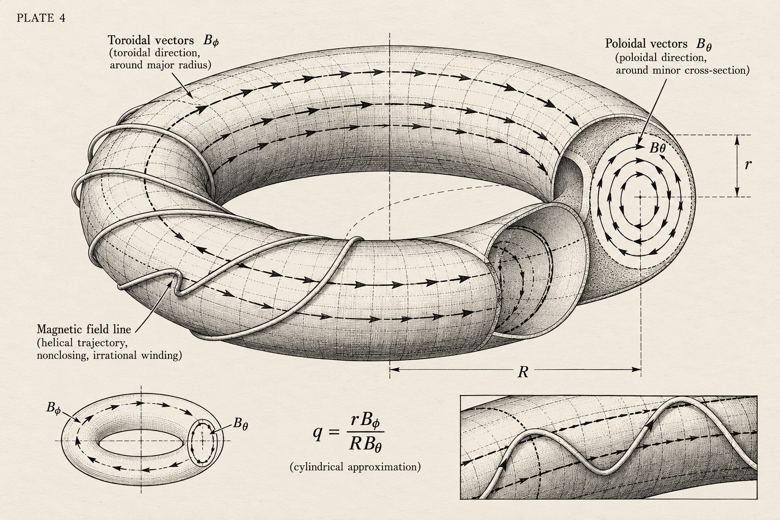
What does measure physically? It measures the number of toroidal turns () a single field line must make around the major axis in order to complete exactly one poloidal turn () around the minor cross-section.
If , the field line wraps once around the big ring for every one turn around the small tube.
If is a rational number (where and are integers), the field line closes back upon its exact starting point after toroidal turns and poloidal turns, forming a closed periodic loop.
If is an irrational number, the field line never closes upon itself; instead, a single continuous trajectory winds ergodically and densely over the entire two-dimensional surface of the torus, knitting the whole shell into an unbroken fabric.
(As conscientious physicists, we remind the reader that is an asymptotic large-aspect-ratio approximation, not a universal identity independent of cross-sectional shaping, and that magnetic flux surfaces are mathematical loci of field-line tangency rather than solid brick walls—actual charged particle gyro-orbits, fluid drift velocities, and heat transport deviate slightly from field lines and must be tracked separately.)
Pause and marvel at the philosophical correspondence that emerges directly from this plasma equilibrium condition. If a practitioner tries to live a purely "worldly" life—marching endlessly around the major toroidal ring of commercial transactions () while reducing his inward poloidal turn of silent reflection to zero (, so )—the vertical drifts of unexamined stress and reactivity go uncompensated, and his life is hurled outward against the wall. Conversely, if he tries to live exclusively in an isolated inward loop () without sufficient longitudinal stabilization along the major ring of worldly livelihood, his containment pinches off into violent local sausage and kink instabilities (the classic Kruskal-Shafranov limit, requiring at the boundary for stability).
Stability requires a finite, non-zero helical pitch: the steady, simultaneous marriage of toroidal livelihood () and poloidal recollection ().
| Geometric / Physical Feature | Mathematical Expression | Useful Contemplative & Practical Correspondence | Dualistic Misinterpretation to Avoid |
|---|---|---|---|
| One surface, two orthogonal angles | Two complementary aspects of one undivided lived activity (inward reflection and outward service ). | Calling and a strict mathematical identity for the Two Truths. | |
| A family of dependent nested surfaces | Processes of regulation operating concurrently across household, lab, and mind at different scales. | Imagining an "inner ultimate substance" locked inside a shell of "outer false appearances". | |
| Helical winding and the safety factor | The necessary rhythmic return between marketplace engagement and quiet attentional grounding. | Assuming that every psychological state or life event is mechanically periodic. | |
| The central opening of the torus | Throat region | A visible topological feature allowing continuous recurrence without a dead-end pole. | Labeling the physical hole śūnyatā or worshipping it as a localized cosmic battery. |
2.4 Resistive Magnetohydrodynamics and the Energy Budget of Livelihood
To see how the field and the living medium actually push and pull upon one another over time, we must move from static geometry to the dynamical equations of resistive magnetohydrodynamics (MHD).
Consider an electrically conducting fluid of mass density , bulk fluid velocity , scalar kinetic pressure , electrical conductivity , and constant magnetic diffusivity . Combining Maxwell’s pre-relativistic equations (Ampère’s law , Faraday’s law of induction , and the absence of magnetic monopoles ) with Ohm’s law for a moving conductor (), we eliminate the electric field to obtain the foundational MHD Induction Equation:
Simultaneously, the fluid velocity evolves according to the MHD Momentum Equation (the Navier-Stokes equation augmented by the electromagnetic Lorentz force):
where is the dynamic fluid viscosity and represents external gravitational or mechanical forcing.
Look closely at the two right-hand terms of the induction equation:
1. The Convective Coupling Term, : This term couples magnetic evolution directly to fluid motion. In the ideal MHD limit where electrical resistivity vanishes (), Alfvén’s Flux-Freezing Theorem holds: magnetic field lines are "frozen into" the conducting fluid and are carried along with like dye threads in water. In this ideal limit, the topology of the field is strictly locked; linked loops cannot untie themselves, and new nested loops cannot be torn open.
2. The Resistive Diffusion Term, : In any real laboratory plasma or natural fluid, is finite. Resistivity allows the magnetic field to slip across the fluid, smoothing out sharp current gradients and—most importantly—permitting magnetic reconnection across thin current sheets. Because of finite resistivity , topology is not frozen in stone: separate flux loops can merge, and newly injected loops can splice smoothly into the primary circulation.
At the same time, finite resistivity and fluid viscosity exact an unavoidable thermodynamic price. If we integrate the total stored magnetic and kinetic energy inside the toroidal volume :
and take its time derivative using the MHD equations, we arrive at the global Energetic Balance Equation:
Here, represents the rate of organized power injected across the system boundaries (via electromagnetic induction, neutral beam injection, or mechanical pumping), represents organized work or radiation exported by the system, and is the strictly positive rate of irreversible dissipation:
which continuously converts organized field and flow energy into random thermal heat via Ohmic resistance () and viscous friction ().
This simple equation, , is a cold bucket of spring water thrown in the face of every romantic pseudo-mystic who claims that because the universe is a torus, a spiritual person should be able to live on "free cosmic energy" without working, eating, or paying his laboratory rent!
Recirculation is not creation ex nihilo. A toroidal geometry allows a system to retain, organize, and recirculate energy with extraordinary efficiency rather than letting it shoot off to infinity in a straight line—just as a flywheel or a regenerating catalytic loop conserves momentum or cofactors. But sustained operation in a resistive universe always requires an honest energy budget ().
In the human domain, is the daily metabolic burn of neurons and muscle tissue, the wear and tear on shoes and glassware, the entropy of a household roof in winter. is the useful technical service delivered to clients and the care given to loved ones. And is the clean intake of food, rest, quiet breath, and fair monetary payment received for useful work. To respect the energy budget is not materialism; it is honoring the conservation laws of the very medium through which awareness moves.
2.5 The Formal Theory of "Superinsertion"
We are now equipped to define the central operational term of this book. As noted in the Preface, the word superinsertion does not appear in standard 1978 textbooks of plasma physics or control engineering; we introduce it here as a rigorous technical coinage to bridge multi-scale field mechanics, biochemical network design, and contemplative practice.
Definition (Superinsertion): Superinsertion is the controlled introduction of an additional recurrent process into an existing network of recurrent processes, accompanied by non-zero cross-scale coupling that alters, stabilizes, or regenerates the subsequent dynamical behavior of the composite network.
Let us write the general state-space formalism for superinsertion before examining its magnetic and chemical special cases.
Suppose we have an established primary recurrent system described by an -dimensional state vector , evolving according to an autonomous nonlinear vector field that possesses a stable periodic orbit or toroidal attractor . Left to itself under external environmental disturbances , the primary cycle evolves as:
Suppose that under heavy load or dissipative drain, this primary loop suffers from drift, cofactor depletion, or high-frequency turbulence. Instead of attempting to brute-force back on track through massive external forcing , we introduce a secondary, compact recurrent process described by an -dimensional state vector , whose uncoupled internal dynamics execute a rapid, self-contained cycle .
We superinsert into by opening two bidirectional coupling channels governed by coupling functions and with coupling constants and :
Notice immediately what scientific honesty requires us to state about this coupled system: Merely writing down coupled differential equations does not automatically guarantee nested spatial tori, beneficial feedback, or stable oscillation! Depending on the eigenvalues of the Jacobian matrix of the coupled system:
an ill-chosen coupling can just as easily drive a stable system into destructive resonance, phase-locking paralysis, or chaotic blow-up. For superinsertion to succeed as a stabilizing architecture, three strict dynamical conditions must be satisfied:
1. Kinematic Admissibility (Divergence-Free Insertion): In a continuous field system such as a magnetized plasma, any newly superinserted magnetic loop added to a background field () must preserve the solenoidal constraint everywhere. We guarantee this kinematically by introducing the perturbation through a smooth vector potential such that:
Wherever the second partial derivatives of are continuous, the vector identity is satisfied automatically.
2. Resistive Topological Handshake (Reconnection Window): As we saw in Alfvén’s flux-freezing theorem, if the background medium is rigidly frozen (), an externally injected flux loop cannot link with the interior nested surfaces ; it merely bounces off the outer skin like a rubber ball off a drumhead. Successful superinsertion requires a localized window of finite diffusivity () at the boundary layer where the injected loop and the primary ring meet, allowing the field lines to reconnect and knit into a single shared topology before relaxing back into low-dissipation flow.
3. Dissipative Phase-Matching ( Sign Condition): The cross-coupling terms and must be phased such that the fast internal loop absorbs excess turbulent variance from the slow outer loop (or regenerates the specific state variable that consumes), rather than pumping positive-feedback noise into ’s unstable modes.
Let us see how this single mathematical structure—the coupled equations of superinsertion—manifests across the three practical laboratories of our treatise:
In Toroidal Plasma Physics (Spheromak / Flux-Core Injection): is the primary toroidal confinement ring inside the vessel; is a compact magnetized plasma ring generated by a coaxial gun and injected into the torus, where resistive reconnection splices its helicity into the main field, replenishing the poloidal flux against resistive decay.
In Cell-Free Biochemical Engineering (Chapter 4): is the primary enzymatic synthesis cascade converting precursor substrates into target alkaloid products while consuming high-energy cofactors (such as ATP or NADH); is the auxiliary enzymatic regeneration loop superinserted into the same reactor vessel, coupled via shared cofactor intermediates so that spent ADP/NAD is continuously re-energized without requiring a living cell.
In the Conduct of an Embodied Life (Chapters 3, 5, and 6): is the outer macro-circuit of saṃvṛti-satya—the weekly revolution around the major angle of commercial consulting, laboratory trials, contract negotiation, invoicing, and household chores. Left uncoupled (), gradually accumulates egoic friction, defensive insistence, and attentional exhaustion. is the rapid, silent poloidal turn () of non-dual recollection—ten minutes sitting quietly on a storeroom stool between drums of maltodextrin, dropping self-description, and holding the universe concise. When is superinserted into the middle of Wednesday afternoon (), the silence does not abolish the chemistry; it clears the phase-space of so the chemist can return to the bench and notice the batch mixing order on line one.
2.6 Constrained Relaxation and the Conservation of Helicity (Taylor’s 1974 Theorem)
There remains one final physical mystery in the mechanics of the supertoroid—a breakthrough achieved just four years ago that bridges field physics and the contemplative discipline of Purge, Unify, Simplify with breathtaking precision.
Throughout the 1950s and 1960s, plasma physicists working on toroidal pinch machines (such as the ZETA apparatus in England) observed a baffling phenomenon. They would strike a violent, turbulent electric discharge inside a toroidal tube filled with ionized gas. Initially, the plasma was a chaotic nightmare of violent kinks, resistive instabilities, and tangled magnetic eddies. Yet within a fraction of a millisecond, instead of disintegrating completely into random thermal gas, the plasma spontaneously quieted down! It shed its violent local turbulence and settled into a remarkably stable, quiescent, symmetric state in which the toroidal magnetic field near the outer wall actually reversed its sign (the Reversed-Field Pinch).
How could a turbulent, dissipative fluid spontaneously organize itself into a quiet, force-free geometry?
In November 1974, the British theoretical physicist J. B. Taylor solved this twenty-year riddle in a three-page paper in Physical Review Letters titled "Relaxation of Toroidal Plasma and Generation of Reverse Magnetic Fields".
Taylor began by examining what happens in a toroidal plasma with a small but finite electrical resistivity () enclosed within a perfectly conducting toroidal shell. Because is non-zero, Alfvén’s ideal flux-freezing constraint is broken at small scales: rapid, fine-scale magnetic reconnection occurs across thousands of tiny turbulent current sheets throughout the plasma. Consequently, the individual nested flux surfaces are temporarily torn and re-knitted, and the total magnetic energy of the system:
is rapidly dissipated as heat ().
In ideal MHD (), there is an infinite number of topological invariants—specifically, the magnetic helicity inside every individual closed flux tube is separately conserved. Magnetic helicity inside a volume is defined as the volume integral of the dot product of the magnetic vector potential and the magnetic field :
Geometrically, magnetic helicity measures the net topological linkage, knotting, and twist of the magnetic field lines with one another (for two simply linked flux tubes carrying fluxes and , their mutual helicity is simply ).
Taylor’s stroke of genius was to compare the relative decay rates of magnetic energy and total magnetic helicity during turbulent resistive reconnection. Because magnetic energy leads to resistive dissipation proportional to , spatial derivatives of are squared; thus, fine-scale turbulent eddies with huge local gradients burn off magnetic energy at an enormous rate. By contrast, the rate of change of total magnetic helicity involves one fewer spatial derivative ().
Therefore, during rapid, small-scale reconnection across the plasma, total magnetic energy decays rapidly toward a minimum, while the global magnetic helicity integrated over the entire toroidal vessel remains almost perfectly conserved!
Let us perform Taylor’s variational calculation explicitly. We seek the magnetic field configuration that minimizes the total magnetic energy subject to the constraint that the global helicity remains fixed at its initial value . Using the method of Lagrange multipliers, we introduce a constant scalar multiplier and set the first variation of the functional equal to zero:
Taking the variation with respect to and integrating by parts (employing the vector identity ) under the boundary condition that the normal component of and tangential electric field vanish on the conducting wall, the volume integral yields the Euler-Lagrange stationarity condition:
For this integral to vanish for all arbitrary admissible variations inside the torus, the integrand itself must vanish identically everywhere! We arrive at Taylor’s Force-Free Relaxation Equation:
where is a uniform spatial constant across the entire relaxed plasma determined solely by the ratio of conserved global helicity to the toroidal magnetic flux.
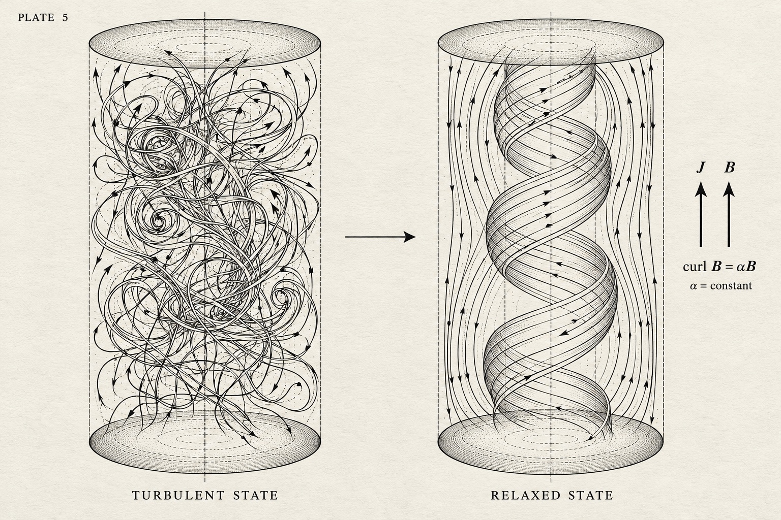
Look at what means physically! By Ampère’s law (), this equation states that throughout the relaxed torus, the electric current density flows strictly parallel to the magnetic field at every point (). And when is parallel to , what happens to the destructive electromagnetic Lorentz force that was tearing the fluid apart?
The cross-field Lorentz force vanishes identically everywhere! In cylindrical coordinates modeling a large-aspect-ratio torus, the solutions to are the classic Bessel Function Model (BFM) fields:
where and are Bessel functions of the first kind—smooth, self-organizing helical waves in which the poloidal and toroidal fields lock into effortless harmonic proportion from the core to the boundary.
Let us state both the power and the boundary of this physical analogy with crystal clarity. Taylor’s theorem does not prove that the human psyche is an ionized hydrogen gas, nor that human morality possesses a magnetic vector potential measured in Webers per meter. What Taylor’s theorem provides is an exact, mathematically rigorous demonstration of a profound systems principle: When a complex circulating system is relieved of the burden of defending every brittle local sub-surface and allowed to relax, it does not collapse into featureless nothingness; it sheds its high-energy parasitic turbulence () while preserving its overarching topological linkage (), settling naturally into a state where flow () and structure () run parallel without internal friction ().
In human terms, we spend half our lives exhausting ourselves trying to preserve every petty local flux surface—every defensive opinion, every half-baked project we promised three years ago, every anxious rehearsal of how our colleagues perceive us. Our internal current (our daily effort and insistence) crosses at right angles against our true field (our actual life conditions and deepest values), generating massive internal Lorentz stress () and Ohmic burnout ().
When we practice constrained relaxation—what our chemist’s workbench card calls Purge, Unify, Simplify—we permit finite resistivity to dissolve those tangled local eddies. Some of the specific small loops we once clung to will indeed change or disappear in the reconnection. Yet the global linkage of our life—our commitment to truth at the laboratory bench, our fidelity to those we love, and our quiet grounding in non-dual awareness ()—survives the purge intact. We emerge in the Taylor state: , where the action of the hands and the stillness of the heart flow along the exact same line.
2.7 Coda: Reading the Equations Without Idolatry
Before we leave the blackboard of Chapter 2 and walk out into the heat of the California desert in Chapter 3, let us post one final guard at the door of the mathematics.
In the exhilarating climate of 1978, when physicists and mystics gather over wine in San Francisco or tea in Big Sur, there is a recurring temptation to commit what Alfred North Whitehead called the Fallacy of Misplaced Concreteness—or what we might call geometric idolatry. Because the parameterized torus is symmetrical, and because Taylor’s force-free equation is breathtakingly compact, the mind is tempted to bow down to the chalk marks on the slate and proclaim: "Behold! I have proved on the blackboard that the universe is non-dual, and because I know the formula for the safety factor , my rent is paid and my marriage is harmonious!"
Nothing could be further from the truth. A differential equation is a map—a dependent designation (upādāya prajñapti), in Nāgārjuna’s precise phrase. It has no svabhāva of its own. A drawing of a nested torus on a sheet of paper does not circulate a single drop of blood or pay a single technician’s wage.
What the geometry of the supertoroid actually resolves for us is a crippling representational bottleneck in our culture. For centuries, whenever a scientist or artisan felt the pull of timeless contemplation alongside the pull of worldly work and domestic love, the only mental pictures available to him were images of division: two rival kingdoms, a soul trapped in a clay cage, a zero-sum seesaw where lifting one end forces the other into the mud.
The supertoroid replaces that broken seesaw with a working dynamic portrait of persistence through relationship. It shows us visually and analytically how:
Multiple scales of circulation () can nest without colliding;
Two orthogonal vectors of movement—inward recollection () and outward marketplace engagement ()—are required simultaneously to generate a stable helical trajectory ();
A closed organizational pattern can endure only by honoring an open thermodynamic energy budget ();
A fresh, ungrasping insight or contemplative pause () can be superinserted into the middle of an industrial workflow () to regenerate what the work consumes; and
Releasing local egoic turbulence () allows the whole life to settle into force-free alignment () around its deepest conserved commitments ().
With the geometry of the nested manifold and the equations of field coupling clearly before us, it is time to test the mathematics against raw asphalt, concrete drainage pipes, bruised heels, and human hunger. Let us turn the calendar back six years to the spring of 1972, and follow a young chemist as he walks out of his California door with a folded map and no money in his pocket.
Chapter companion
Chapter 2 sets out the geometric and physical models that give our tradition its name: the concentric nested supertoroid, the coupling of toroidal and poloidal circulations, and J. B. Taylor’s 1974 theorem on plasma relaxation. In our reading, these equations are honored as genuine mathematics within their physical assumptions, and cherished as a luminous visual grammar for how a human life balances inward return with outward movement.
Core teachings
- A toroidal surface and a solid torus are distinct geometric objects that help us picture nested layers of circulation.
- In a toroidal plasma, long-way (toroidal) and short-way (poloidal) fields must work together to keep the plasma from drifting into the wall.
- In a human week, outward work without inward stillness burns out, while inward stillness without outward care drifts from reality.
- Taylor relaxation shows how a turbulent field can shed tearing stresses while preserving its global linkage.
- Physical conservation laws give us a vivid poetic image for endurance, never a laboratory proof of immortality.
In ordinary life
Think of a season when you worked for weeks without a single quiet hour to ask why, or a season when you sat in solitary reflection while avoiding a hard responsibility. The safety factor in Chapter 2 is a way of picturing why both motions are needed to keep a life centered.
Where to test this
Differential equations on a page can intimidate newcomers or tempt readers into thinking our spiritual claims have been proved in a fusion reactor. Whenever we study Chapter 2, we state the physical assumptions plainly and keep the human teaching accessible in ordinary words.
Sources and scope
Magnetohydrodynamics describes ionized gases in magnetic fields. When we bring its language into contemplation, we do so consciously as metaphor.
Questions for reflection
- What happens in your own life when outward action runs for too long without an inward turn of stillness?
- What is the difference between releasing unnecessary mental clenching and ignoring a real problem?
- Which insight in this chapter speaks to you most clearly even when the equations are set aside?